Reading room · Case study · 21 October 2026

Tuning a chatter filter from a DNP3 capture: 26 updates down to 6

A chattering digital input, a breaker auxiliary contact or an alarm with a loose wire, can flood a SCADA with state changes, fill event buffers and bury the alarms that matter. Every SCADA has a chatter filter; the hard part is choosing its parameters without either hiding real operations or letting the noise through. A capture of the actual updates answers that question with numbers.

The point

Outstation 7 on 10.0.2.7:20000 reports 16 binary inputs. Input 7, breaker CB-7, changes state 12 times in about two seconds every 10 minutes; the other inputs change once every 45 minutes or so. Over 30 minutes CB-7 sends 26 updates, more than all the other digital points together.

A chatter filter, in three parameters

Count: how many transitions are tolerated.
T1: the window in which they are counted.
T2: how long the point is blocked once the count is exceeded. Updates during the block are dropped and the value in the SCADA holds still.

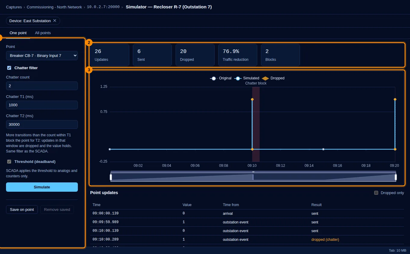
Simulator chart for breaker CB-7: original line, simulated line, dropped updates and two chatter blocks — Count 2, T1 1000 ms, T2 30000 ms on CB-7: of 26 updates, 6 reach the SCADA and 20 are dropped, in 2 blocks. The dashed line is what the outstation sent, the solid line what the SCADA would show.

With count 2, T1 1 s and T2 30 s, each burst passes its first transitions, trips the filter and is blocked for the rest: 20 of 26 updates dropped, a 76.9% reduction, in two blocks. The final state after each burst still gets through when the block ends, so the SCADA does not end up showing a stale position.

A chattering breaker is the easy case, though: it flashes on the operator's screen and floods the alarm list, so someone notices it within minutes. The load that goes unnoticed comes from measurements.

The load nobody sees: a measurement with a tight deadband

The same outstation reports four feeder currents. They come from the protection relay of each feeder bay, an IED that measures the phase current through the bay's current transformers and publishes it in DNP3, read by the substation RTU or gateway. At commissioning their deadband was set to 1 A "to be safe": on a feeder carrying around 210 A that is under 0.5% of the range, and ordinary load noise crosses it all the time. The relay reports a new value about every 10 seconds per point: Analog Input 0 alone sends 178 updates in 30 minutes, and the four together over 700. It is a measurement, not a state: it changes no topology, raises no alarm, every value looks right on a display, and the operator has no reason to look.

Now put an ADMS (advanced distribution management system) behind the SCADA. Its network applications live on measurements: the state estimator reconciles every current and voltage with the network model, and these bay currents are exactly its inputs, and the power flow, load allocation and loss calculations run on its result. An ADMS that re-evaluates when measurements change, or on a short cycle that a steady stream of changes keeps busy, spends that effort on noise: one feeder current changing by a fraction of an ampere is a new estimation input, a new solution, new values pushed to every display and historian downstream. Multiply by every feeder measurement with a deadband set "to be safe", and the analysis applications and the SCADA's own data processing carry a load that no single point explains.

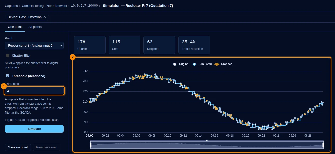
Simulator threshold view for the feeder current: 178 updates, 115 sent, 63 dropped with a threshold of 2 — A threshold of 2 A on the feeder current, 3.7% of its recorded range of 183 to 237 A: of 178 updates, 115 are sent and 63 dropped (35.4% less traffic), and the simulated line follows the real load curve.

Replaying the real updates through a deadband shows what a better setting buys before you change anything in the field: with 2 A instead of 1 A, 35% fewer updates reach the SCADA, and the curve the ADMS works with keeps its shape. The capture turns "the system is slow" into a ranked list of which points send the most for the least information.

Which points need a filter at all

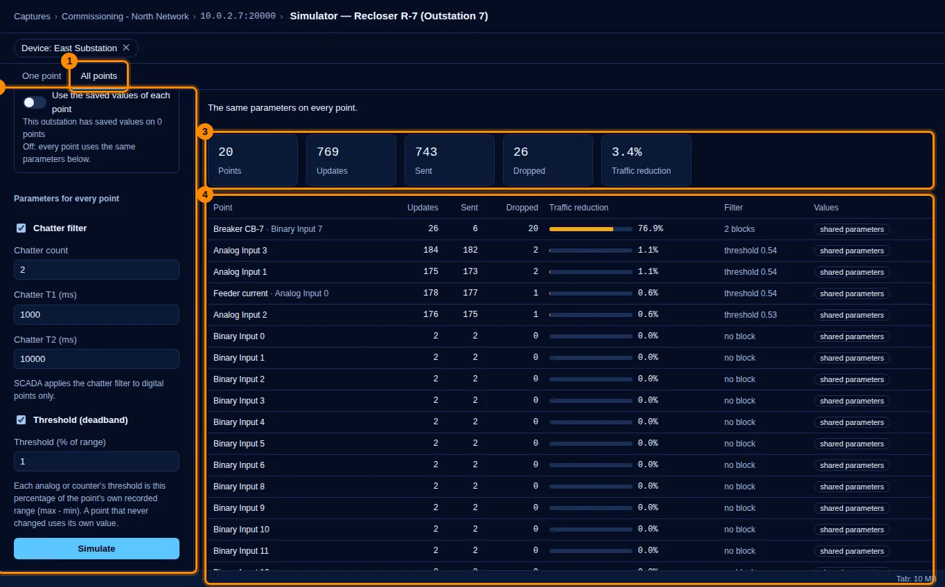
All points simulated at once, ranked by dropped updates, with CB-7 on top — The same parameters applied to every point of the outstation: CB-7 alone accounts for 20 of the 26 dropped updates; the calm inputs lose nothing.

Running the same filter across every point of the outstation is the useful second step: 20 points, 769 updates, 26 dropped, and 20 of those on CB-7. The calm inputs lose nothing, which confirms the parameters do not hide genuine operations. The analog points are filtered by a deadband instead (1% of each point's recorded range here), which trims only one or two readings each.

Rules of thumb

Choose T1 from the chatter itself: a little longer than the time a burst takes.
Choose T2 from operations: shorter than the time an operator would wait before acting on a stale position.
Check the result on every point with the same parameters, not just the noisy one.
For measurements, size the deadband from the recorded range and the noise, not from habit; look at the busiest analogs first.
Fix the contact. The filter is a mitigation; the capture is also the evidence for the maintenance ticket.
Related: what a self-healing (FLISR) scheme needs from the same DNP3 traffic.

Try it on your own capture

ComputingSphere DNP3 decodes a pcap once, splits it per channel and per outstation, and ranks the outstations worst first with the same numbers used here. It only reads what already went over the wire. The Simulator replays each point’s real updates through the same chatter and deadband filters ComputingSphere SCADA applies. This capture is among the examples of every free account, to reproduce every number in this post; or upload your own: the Free plan covers 1,000 messages a month.